
")
Cover Image Credit: Synth
High-quality price path predictions are not judged solely by where prices end up. What matters just as much is how uncertainty evolves over time. For trading systems, intra-day risk management, and derivative pricing, the structure of volatility is often more important than directional accuracy.
This is where volatility autocorrelation becomes essential.
In real markets, volatility does not behave randomly; it clusters. Periods of high volatility tend to persist, as do periods of calm. Any predictive system that aims to model realistic price dynamics must capture this temporal structure.
Synth, subnet 50 on bittensor, provides a useful case study in how incentive-driven forecasting can internalize these dynamics at scale.
Why Volatility Autocorrelation Matters
Volatility autocorrelation measures whether current volatility contains information about future volatility. The standard approach uses squared returns as a proxy for instantaneous volatility and examines how those values correlate across time lags.
Positive autocorrelation indicates persistence. If volatility is high now, it is likely to remain elevated in the near future. Negative autocorrelation at longer horizons signals mean reversion, ensuring volatility does not drift indefinitely.
For intraday forecasting and execution, this structure is not optional. Without it, predicted price paths may look plausible at the endpoint while behaving unrealistically along the way.
Miner-Level Volatility Persistence at Short Horizons
Using Synth miner predictions at a five-minute resolution, the autocorrelation of squared returns reveals a clear and coherent volatility memory.
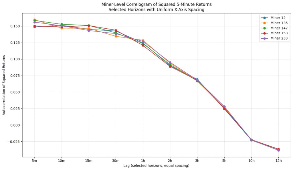
At the shortest horizon, corresponding to a single five-minute lag, autocorrelation values cluster tightly around 0.15 to 0.16. This is a strong signal of persistence. When volatility spikes, it does not disappear in the next interval. Shocks carry forward momentum.
As the horizon extends, autocorrelation decays smoothly rather than abruptly.
Key observations include:
a. Around 30 minutes, autocorrelation remains near 0.14,
b. At 1 hour, it declines modestly to roughly 0.12 to 0.13, and
c. By 3 hours, it falls further to around 0.07.
This gradual decay reflects diminishing memory. Past volatility still matters, but its influence weakens steadily over time.
By approximately 5 hours, autocorrelation approaches near zero. At this point, the market has largely forgotten the original shock.
At even longer horizons, autocorrelation turns mildly negative. Values around minus 0.02 to minus 0.04 appear between 10 and 12 hours, indicating mean reversion. Elevated volatility becomes slightly more likely to be followed by lower volatility, anchoring the system around a stable intraday level.
Notably, miner curves are nearly indistinguishable across all horizons. This tight alignment suggests miners are converging on a shared volatility structure rather than producing idiosyncratic dynamics.
How Autocorrelation Appears in Forward Volatility
The forward volatility curve provides a visual counterpart to the correlogram. Volatility at each five-minute step is computed from the ensemble of predicted paths, offering a forward looking view of uncertainty.
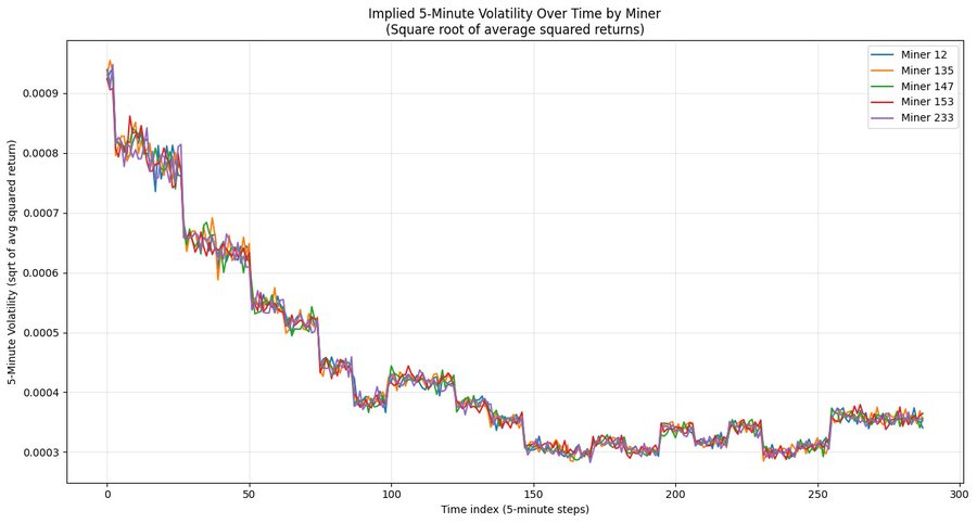
At the beginning of the horizon, implied volatility is elevated, around 0.0009 to 0.00095. This directly reflects the strong short-term autocorrelation. Because volatility is persistent, it decays gradually rather than collapsing.
Over the first hour, volatility declines toward 0.0006 to 0.00065, mirroring the reduction in autocorrelation from roughly 0.16 toward the low 0.12 range. Beyond that point, the curve continues to flatten as autocorrelation approaches zero.
Later in the horizon, volatility stabilizes around 0.0003 to 0.00035. This plateau corresponds to the region where autocorrelation becomes negligible and then mildly negative. Mean reversion prevents volatility from drifting lower and enforces convergence.
In effect, the correlogram explains why the volatility curve is smooth, persistent, and ultimately stable. The forward plot shows how that structure unfolds through time.
What This Reveals About Synth Miner Predictions
Taken together, these results demonstrate that Synth miners are learning more than point estimates or terminal outcomes. They are encoding second-order temporal structure.
The predictions capture:
a. Short-term volatility persistence,
b. Gradual decay of volatility memory, and
c. Long horizon mean reversion.
The near-perfect alignment across miners indicates that Synth’s scoring and incentive mechanisms are actively enforcing realistic market behavior.
The result is not a collection of independent forecasts, but a coherent stochastic process with well-defined volatility dynamics.
This kind of temporal consistency is essential for practical applications. High frequency execution, intraday risk control, and derivative pricing all depend on how uncertainty evolves, not just where prices land.
Conclusion
Volatility autocorrelation provides a powerful lens for evaluating the realism of predicted price paths. In the case of Synth, it reveals a system that internalizes key features of real market behavior, including clustering, persistence, and mean reversion.
By aligning miner incentives around these dynamics, Synth produces forecasts that behave like markets rather than simulations. That distinction is subtle, but it is exactly what separates toy models from production-ready financial intelligence.In short, Synth miners are not just predicting prices. They are learning how markets remember, forget, and stabilize uncertainty over time.


Be the first to comment